This post was developed to show the use of HEC-DSSVue for viewing the results of HEC-ResSim. Using HEC-DSSVue may be preferable for exporting data to Microsoft Excel or for developing custom plots with specified parameters.
For this example, I developed a simple model with one reservoir. The model layout is shown below.

For this model, I added a constant seepage from the pool of 5 cfs. The dam has two outlet groups. "Outlet Group a" has one controlled outlet with a capacity of 500 cfs. "Outlet Group b" has two controlled outlets. These outlets have a smaller capacity with "a" having a capacity of 15 cfs, and "b" having a capacity of 20 cfs. The physical data is shown below.

The top of conservation pool is set at 80 ft. There are no rules in this model. The operational data is shown below.

With the simulation starting at a pool elevation of 87 ft, the simulation begins in the flood pool. The total capacity of 535 cfs is used to bring the pool down to the top of conservation. Once there, the inflow (minus the seepage of 5 cfs) is passed to hold top of conservation. For this simulation a constant inflow of 475 cfs enters the model at the upstream end.

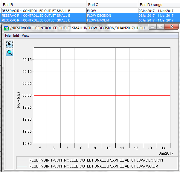
To access the results in HEC-DSSVue, the user selects HEC-DSSVue under the Tools menu in the Simulation Module. In the figure below, two DSS paths are selected and plotted. The C part of "FLOW-DECISION" and "FLOW-MAXLIM" are plotted for the large outlet in group A. The "FLOW-MAXLIM" of 500 cfs is shown with the red line. In emptying the flood pool, the total capacity of this outlet is used. Once the top of conservation is reached, the flow going through this outlet is reduced to the amount needed to pass inflow and hold top of conservation. This outlet passes 435 cfs while the smaller outlets are maxed out at 35 cfs combined (shown in figures that follow) to hold top of conservation. The 470 cfs going through the outlets plus the 5 cfs of seepage holds top of conservation since this amounts equals inflow.

For the outlet "a" in outlet group B, the flow going through this outlet is set to its maximum of 15 cfs for the entire simulation. Note that the plots for "FLOW-DECISION" AND "FLOW-MAXLIM" are coincident in the figure below.

For the outlet "b" in outlet group B, the flow going through this outlet is also set to it maximum of 20 cfs for the entire simulation. Note that the plots for "FLOW-DECISION" AND "FLOW-MAXLIM" are coincident in the figure below.

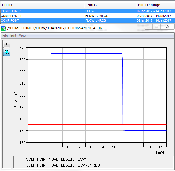
In the figure below, the total inflow (blue line) is 475 cfs for the entire simulation. The net inflow (red line) is 470 cfs for the entire simulation since seepage is subtracted from total inflow to compute net inflow. Note that net inflow is computed for the simulation which begins on 05Jan2017. The lookback period begins on 03Jan2017 for this simulation.

The junction, "COMP POINT 1", has an unregulated flow (flow as if the dam is not in place) that is equal to the inflow. Note that the unregulated flow is higher than the computed flow at that junction once inflow is being passed since seepage that is lost to the system is not passed through the dam. Seepage would not have occurred without the dam in place so that is not subtracted in the computation of unregulated flow.

To show the difference between seepage and leakage, I performed an additional simulation where I changed the seepage to zero and added leakage of 5 cfs. As stated above, seepage is removed from the system, however, leakage is released into the tailwater and continues downstream. Because of this, the computed flow at the junction, "COMP POINT 1", is 5 cfs higher than the simulation which included seepage.

For this example, I developed a simple model with one reservoir. The model layout is shown below.

For this model, I added a constant seepage from the pool of 5 cfs. The dam has two outlet groups. "Outlet Group a" has one controlled outlet with a capacity of 500 cfs. "Outlet Group b" has two controlled outlets. These outlets have a smaller capacity with "a" having a capacity of 15 cfs, and "b" having a capacity of 20 cfs. The physical data is shown below.

The top of conservation pool is set at 80 ft. There are no rules in this model. The operational data is shown below.

With the simulation starting at a pool elevation of 87 ft, the simulation begins in the flood pool. The total capacity of 535 cfs is used to bring the pool down to the top of conservation. Once there, the inflow (minus the seepage of 5 cfs) is passed to hold top of conservation. For this simulation a constant inflow of 475 cfs enters the model at the upstream end.

To access the results in HEC-DSSVue, the user selects HEC-DSSVue under the Tools menu in the Simulation Module. In the figure below, two DSS paths are selected and plotted. The C part of "FLOW-DECISION" and "FLOW-MAXLIM" are plotted for the large outlet in group A. The "FLOW-MAXLIM" of 500 cfs is shown with the red line. In emptying the flood pool, the total capacity of this outlet is used. Once the top of conservation is reached, the flow going through this outlet is reduced to the amount needed to pass inflow and hold top of conservation. This outlet passes 435 cfs while the smaller outlets are maxed out at 35 cfs combined (shown in figures that follow) to hold top of conservation. The 470 cfs going through the outlets plus the 5 cfs of seepage holds top of conservation since this amounts equals inflow.

For the outlet "a" in outlet group B, the flow going through this outlet is set to its maximum of 15 cfs for the entire simulation. Note that the plots for "FLOW-DECISION" AND "FLOW-MAXLIM" are coincident in the figure below.

For the outlet "b" in outlet group B, the flow going through this outlet is also set to it maximum of 20 cfs for the entire simulation. Note that the plots for "FLOW-DECISION" AND "FLOW-MAXLIM" are coincident in the figure below.
In the figure below, the total inflow (blue line) is 475 cfs for the entire simulation. The net inflow (red line) is 470 cfs for the entire simulation since seepage is subtracted from total inflow to compute net inflow. Note that net inflow is computed for the simulation which begins on 05Jan2017. The lookback period begins on 03Jan2017 for this simulation.

The junction, "COMP POINT 1", has an unregulated flow (flow as if the dam is not in place) that is equal to the inflow. Note that the unregulated flow is higher than the computed flow at that junction once inflow is being passed since seepage that is lost to the system is not passed through the dam. Seepage would not have occurred without the dam in place so that is not subtracted in the computation of unregulated flow.
To show the difference between seepage and leakage, I performed an additional simulation where I changed the seepage to zero and added leakage of 5 cfs. As stated above, seepage is removed from the system, however, leakage is released into the tailwater and continues downstream. Because of this, the computed flow at the junction, "COMP POINT 1", is 5 cfs higher than the simulation which included seepage.

Comments
Post a Comment