Microsoft Excel Basic #3 - Anchoring a cell to be used in computations

In Excel, sometimes it is necessary to anchor a cell for use in computations.  Recall that Excel automatically increments the row or the column number when applying a formula to multiple cells.

In the example below, we want to add the number in cell B8 to the numbers in cells A2 through A6 by applying a formula in cells B2 through B6.

We start by writing the following equation in cell B2:  =A2+B8

The result is shown below.

This result is correct, however we encounter a problem when we drag the equation down to cells B3 through B6.  Excel increments the row number by 1 in each cell, but there are no values in cells B9 through B12 so the result is incorrect since Excel adds zero instead of one.  This is demonstrated below.

To correctly apply this formula to each cell, we anchor the row number with the $ symbol.   

In cell B2, we write the following equation:  =A2+B$8.  This will anchor the row number so that Excel does not increment it.  This is shown below:

When we drag this formula to cells B3 through B6, we now get the correct answers as shown below:

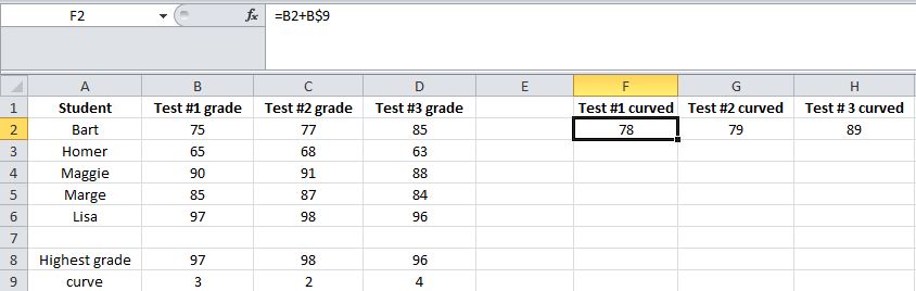
We can refer back to our grades example to apply this concept.  If we wanted to curve the grades for each test based on scaling the highest grade up to 100, we can develop a curves result by subtracting the highest grade from 100.  The curves are shown in cells B9 through D9.  The curved grades will be shown in cells F2 through H6.  In cell F2, we write the equation, =B2+B$9.  This is shown below.

For curving Test #2, we write the equation, =C2+C$9, in cell G2.  This is shown below.  Note that cell H2 contains the equation, =D2+D$9 for curving Test #3.

When these equations are dragged down to cells F3 through H6, the row number is not incremented.  The results are shown below.  It can be seen that Test #1 grades are increased by 3 points, Test #2 grades are increased by 2 points, and Test #3 grades are increased by 4 points.