This post will demonstrate how to determine if a value in one column is present in another column.
This post will revisit the MATCH function in Excel (see Microsoft Excel Advanced #1 for more information) and introduce the ISERROR function. Additionally, the use of IF and NOT will be shown.
The coding for a simple IF statement is as follows:
IF(logical_test,[value_if_true],[value_if_false])
A simple example is shown below where the value in cell A1 is examined. In this example, if cell A1 has a value of 1, then Excel will print "The value is 1". If cell A1 has a value of something other than 1, then Excel will print "The value is not 1". The coding is shown below. For our example, this is entered into cell C1.
The results with cell A1 equal to 1 and cell A1 not equal to 1 are shown below.


For the logical test in the example above, we tested whether cell A1 had a value of 1.
We can use the ISERROR function as our logical test. In this case we will determine whether or not a computation is possible in cell A1. For example, a computation of 2+1 is possible, however, 2/0 is not possible since we are dividing by zero.
The coding is shown below:
Entering the formula =2+1 into cell A1 gives the following result:
Entering the formula =2/0 into cell A1 gives the following result:

The MATCH function searches for a specific item in a range of cells, and then returns the relative position of that item in that range. It is coded as follows:
MATCH(lookup_value,lookup_array,[match_type])
For match_type of 1, Excel finds the largest value that is less than or equal to the lookup_value. To use this, the lookup_array must be in ascending order.
For match_type of 0, Excel finds the first value that is exactly equal to the lookup_value. The values in lookup_array can be in any order.
We can use the MATCH function as our argument in the ISERROR function. We will have Excel look at each individual value in a column and test whether or not it exists anywhere in a different column.
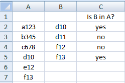
In this case we compare the values in columns A and B. The two columns of data are shown below.

We will write our formula in column C. We will be testing if the values in column B are in column C. In cell C2 we write the following formula:
The zero in the MATCH function means that Excel will be looking for an exact match. If it does not find an exact match, the ISERROR function returns a FALSE. If it does find an exact match, the ISERROR returns a TRUE. Remember to anchor the rows in the array from cell A2 to A7 so that when you copy the cells to the other rows, that array remains constant.
Below are the results of applying our formula in column C. We can see that the d10 and f13 are in both column A and column B while d11 and f12 are only in column B.

Using the ISERROR function along with an IF statement can sometimes be confusing based on ISERROR returning TRUE and FALSE. Basically, the outputs from your IF statement can appear reversed. If you prefer, you can add a NOT after the IF and change the order of the outputs from the IF statement. This is shown below:
The result remains the same:
Comments
Post a Comment