Microsoft Excel Advanced #1 - Introduction to Index and Match functions

I have used the INDEX and MATCH functions to determine a y-value (dependent variable) based on a given x-value (independent variable).  I will demonstrate this in a follow-up post.  This post will serve as an introduction to the use of the INDEX and MATCH functions.

The INDEX function returns the value of an element in a table or an array, selected by the row and column number indexes.  It is coded as follows:

INDEX(array,row_num,column_num)

Row_num will select the row in the array from which to return a value.  If row_num is omitted, column_num is required.

Column_num will select the column in the array from which to return a value.  If column_num is omitted, row_num is required.

For this example, the following set of x and y values is used.  For this post, we will only be dealing with the x values.

We use the INDEX function in cell D2.  For this example, we specify the array as being A2:A11.  The row_number we are looking for is row number 6.  Note that row 1 starts in cell A2 since our array is from A2:A11.  In our example, we omit the column number since it is not needed for our purposes.  Since the value of 60 is in the sixth row, that is the value that populates cell D2.  This is shown in the figure below.

The MATCH function searches for a specific item in a range of cells, and then returns the relative position of that item in that range.  It is coded as follows:

MATCH(lookup_value,lookup_array,[match_type])

For match_type of 1, Excel finds the largest value that is less than or equal to the lookup_value.  To use this, the lookup_array must be in ascending order.

For match_type of 0, Excel finds the first value that is exactly equal to the lookup_value.  The values in lookup_array can be in any order.

Excel also has a match type for a list in descending order.  For this example, we will be showing match_type of 0 and 1.  In the image below, we use the MATCH function in cell D2.  We specify a lookup_value of 30, a lookup_array of A2:A11, and a match_type of 0.  This function returns a value of 3 since 30 is in the third row of A2:A11.

For the next example, we specify a lookup value of 35 and a match_type of 1.  Since the function will return the position of the largest value that is less than or equal to the lookup value it returns 3 since 30 is the largest value in A2:A11 that is less than 35.  This is shown below in cell D2.

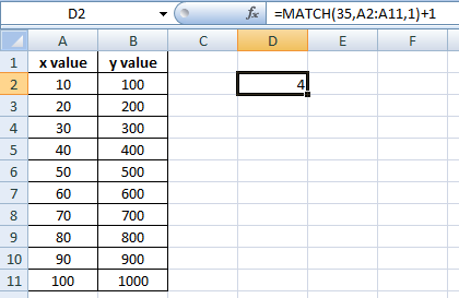
We may need to find the position that is both below and above our lookup_value.  To find the position above our lookup_value, we can simply add 1 to the MATCH function that we used above.  This is shown in the figure below in cell D2.

A follow-up post will show how to combine these functions to extract the values needed for determining a y-value based on a given x-value.